Building Virtual Worlds, Part 5

Asynchronous loading is finally working…

After about a month, I’ve finally got the loading of 3D content into the data cache working asynchronously. It’s taken me a lot of work to get this right as it had to be implemented using double message queues to offload background workers to another thread while the main thread continues with the rendering. Once the 3D content is loaded into the main cache, a message gets pushed back to the rendering thread, signalling that the new block of buildings is ready for display.

It’s a pity that the YouTube clip ends up so blurred, but it might be that it doesn’t like my 21:9 aspect ratio monitor. The original clip is 2560×1080 pixels, so it started out OK.

Now that I’ve got the message queues sorted out I’m going to go back and revisit some of the rendering. The Earth textures also need to load on demand as you can see how I’ve compromised the level of detail above. Also, the buildings don’t load into buffers on the background thread yet. The SSD disk on my machine is so fast that it looks like they’re loading from RAM when actually they’re coming from the disk. Running on my iMac at work shows what a big difference it makes.


3D Buildings

I’ve been experimenting with 3D buildings in my virtual globe project and it’s now progressed to the point where I can demonstrate it working with dynamically loaded content. The following YouTube clip shows the buildings for London, along with the Thames. I didn’t have the real heights, so buildings are extruded up by a random amount and, unfortunately, so is the river, which is why it looks a bit strange. The jumps as it zooms in and out is me flicking the mouse wheel button, but the YouTube upload seems to make this and the picture quality a lot worse than the original:

Performance is an interesting thing as these movies were all made on my home computer rather than my iMac in the office. The green numbers show the frame rate. My machine is a lot faster as it’s using a Crucial SSD disk, so the dynamic loading of the GeoJSON files containing the buildings is fast enough to run in real time. The threading and asynchronous loading of tiles hasn’t been completed yet, so, when new tiles are loaded, the rendering stalls briefly.

On demand loading of building tiles is a big step up from using a static scene graph. The way this works is to calculate the ground point that the current view is over and render a square of nine tiles centred on the viewer’s ground location. Calculation of latitude, longitude and height from 3D Cartesian coordinates is an interesting problem that ends up having to use the Newton-Raphson approach. This still needs some work as it’s obvious from the movies that not enough content ahead of the viewer is being drawn. As the view moves around, the 3×3 grid of ground tiles is shuffled around and any new tiles that are required are loaded into the cache.

Working on the principle that tiles are going to be loaded from a server, I’ve had to implement a data cache based on the file URI (just like MapTubeD does). When tiles are requested, the GeoJSON files are moved into the local cache, loaded into memory, parsed, triangulated using Poly2Tri, extruded and converted into a 3D mesh. Based on how long the GeoJSON loading is taking on my iMac, a better solution is to pre-compute the 3D geometry to take the load off of the display software. At the moment I’m using a Java program I created to make vector tiles (GeoJSON) out of a shapefile for the southeast of England. I’ve assumed the world to be square (-180,-180 to 180,180 degrees) then cut the tiles using a quadtree system so that they’re square in WGS84. Although this gives me a resolution problem and non-square 3D tiles, it works well for testing. The next step is to pre-compute the 3D content and thread the data loading so it works at full speed.

Finally, this was just something fun I did as another test. Earth isn’t the only planet, other planets are available (and you can download the terrain maps)…


Tiling the Blue Marble

Following on from my last post about level of detail and Earth spheroids, here is the NASA Blue Marble texture applied to the Earth:

The top level texture is the older composite Blue Marble which shows blue oceans and a very well-defined North Pole ice sheet. Once the view zooms in, all subsequent levels of detail show the next generation Blue Marble from January 2004 with topography [link]. Incidentally, the numbers on the texture are the tile numbers in the format: Z_X_Y, where Z is the zoom level, so the higher the number, the more detailed the texture map. The green lines show the individual segments and textures used to make up the spheroid.

In order to create this, I’ve used the eight Blue Marble tiles which are each 21,600 pixels square, resulting in a full resolution texture which is 86,400 x 43,200 pixels. Rather than try and handle this all in one go, I’ve added the concept of “super-tiles” to my Java tiling program. The eight 21,600 pixel Blue Marble squares are the “super-tiles”, which themselves get tiled into a larger number of 1024 pixel quad tree squares which are used for the Earth textures. The Java class that I wrote to do this can be viewed here: ImageTiler.java. As you can probably see from the GitHub link, this is part of a bigger project which I was originally using to condition 3D building geometry for loading into the globe system. You can probably guess from this what the chunked LOD algorithms are going to be used for next?

Finally, one thing that has occurred to me is that tiling is a fundamental algorithm. Whether it’s cutting a huge texture into bits and wrapping it around a spheroid, or projecting 2D maps onto flat planes to make zoomable maps, the necessity to reduce detail to a manageable level is essential. Even the 3D content isn’t immune from tiling as we end up cutting geometry into chunks and using quad tree or oct tree algorithms. Part of the reason for this rests with the new graphics cards, which mean that progressive mesh algorithms like ROAM (Duchaineau et al) are no longer effective. Old progressive mesh algorithms would use CPU cycles to optimise a mesh before passing it on to the graphics card. The situation now with modern GPUs is that using a lot of CPU cycles to make a small improvement to a mesh before sending it to a powerful graphics card doesn’t result in a significant speed up. Chunked LOD works better, with blocks of geometry being loaded in and out of GPU memory as required. Add to this the fact that we’re working with geographic data and spatial indexing systems all the time and solutions to the level of detail problem start to present themselves.


Links:

NASA Blue Marble: http://visibleearth.nasa.gov/view_cat.php?categoryID=1484

Image Tiler: https://github.com/maptube/FortyTwoGeometry/blob/master/src/fortytwogeometry/ImageTiler.java

ROAM paper: http://dl.acm.org/citation.cfm?id=267028 (and: http://www.cognigraph.com/ROAM_homepage/ )

Building Virtual Worlds

The algorithms required to build virtual worlds like Google Earth and World Wind are really fascinating, but building a virtual world containing real-time city data is something that hasn’t yet been fully explored. Following on from the Smart Cities presentation in Oxford two weeks ago, I’ve taken the agent-based London Underground simulation and made some improvements to the graphics. While I’ve seen systems like Three.js, Unity andOgre used for some very impressive 3D visualisations, what I wanted to do required a lower level API which allowed me to make some further optimisations.

Here is the London Underground simulation from the Oxford presentation:

The Oxford NCRM presentation showed the Earth tiled with a single resolution NASA Blue Marble texture, which was apparent as the view zoomed in to London to show the tube network and the screen space resolution of the texture map decreased.

The Earth texture and shape needs some additional work, which is where “level of detail” (LOD) comes in. The key point here is that most of the work is done by the shader using chunked LOD. If the Earth is represented as a spheroid using, for example 40 width segments and 40 height slices, then recursively divided using either quadtree or octtree segmentation, we can draw a more detailed Earth model as the user zooms in. By using the same number of points for each sub-mesh, only a single index buffer is needed for all LODs and no texture coordinates or normals are used. The shader uses the geodetic latitude and longitude calculated from the Cartesian coordinates passed for rendering, along with the patch min and max coordinates, to get the texture coordinates for every texture tile.

GeoGL_Smartie          GeoGL_WireframeSmartie

The two images above show the Earth using the the NASA Blue Marble texture. The semi-major axis has been increased by 50%, which gives the “smartie” effect and serves to show the oblateness around the equator. The main reason for doing this was to get the coordinate systems and polygon winding around the poles correct.

In order for the level of detail to work, a screen space error tolerance constant (labelled Tau) is defined. The rendering of the tiled earth now works by starting at the top level and calculating a screen space error based on the space that the patch occupies on the screen. If this is greater than Tau, then the patch is split into its higher resolution children, which are then similarly tested for screen space error recursively. Once the screen space error is within the tolerance, Tau, then the patch is rendered.

GeoGL_Earth    GeoGL_OctTreeEarth

The two images above show a correct rendering of the Earth, along with the underlying mesh. The wireframe shows a triangular patch on the Earth at the closest point to the viewer which is double the resolution (highlighted with red line). Octtree segmentation has been used for the LODs.

The code has been made as flexible as possible, allowing all the screen error tolerances, mesh slicing and quad/oct tree tiling to be configured to allow for as much experimentation as possible.

The interesting thing about writing a 3D system like this is that it shows that tiling is a fundamental operation in both 2D and 3D maps. In web-based mapping, 2D, maps are cut into tiles, which are usually 256 pixels square, to avoid having to load massive images onto the web browser. In 3D, the texture sizes might be bigger, but, bearing in mind that Google are reported to be storing around 70TB of texture data for the Earth, there is still the issue of out of core rendering. For the massive terrain rendering systems, management of data being moved between GPU buffers, main memory, local disk and the Internet is the key to performance. My feeling was that I would let Google do the massive terrain rendering and high resolution textures and just concentrate on building programmable worlds that allow exploration, simulation and experimentation with real data.

Finally, here’s a quick look at something new:

VirtualCity

The tiled Earth mesh uses procedural generation to create the levels of detail, so, extending this idea to procedural cities, we can follow the “CGA Shape” methodology outlined in the “Procedural Modeling of Buildings” paper to create our own virtual cities.


Useful Links:

http://tulrich.com/geekstuff/chunklod.html

http://tulrich.com/geekstuff/sig-notes.pdf 

http://peterwonka.net/Publications/pdfs/2006.SG.Mueller.ProceduralModelingOfBuildings.final.pdf

Programmable Maps

GeoGL_Tube

I’ve been getting increasingly frustrated with the tools available to visualise the tube, bus and train data I’ve been collecting, so I’ve ended up creating my own. If you’re wondering why some of the lines don’t have any tubes in the above diagram, it’s because I’ve got the speed set very high and I’m not picking the new route correctly when there is a choice.

The image above is an OpenGL visualisation in C++, but based on my experience with the AgentScript (2D) and Three.js (3D) browser based visualisations. Essentially, I wanted something that would allow me to create the animations that I’ve been using 3DS Max for, but in a much simpler way. The following is a bus animation that I built for a recent presentation:

This was created using 3DS Max, with some custom MaxScript code to load the bus positions and create the animation key frames. The main problem with this is the scale of the data, which is why I had to limit it to between 09:00 and 12:00. Art tools generally don’t like to handle this quantity of data and I’ve also had issues with packages like Unity and Lumion.

Increasingly, I’ve been moving towards the idea of “Programmable Maps” where the visualisation is built through a series of stages which load the data, apply behaviours to elements of the scene that move and produce an impressive 2D or 3D visualisation with advanced lighting or tilt shift in the same way as ViziCities. The use of APIs and 3rd party libraries to obtain the real-time data, along with the temporal aspect, makes it very difficult to fit this type of visualisation into a conventional GIS framework.

The example above is built around a C++ and OpenGL graphics engine, but one that is linked with geospatial libraries so it’s more than just a game engine rendering 3D assets as artwork. The experience with the XBox tubes demo (C#, XNA) and Chrome Three.js example showed that it’s a nightmare to get the geometry in the correct place and orientation unless it’s properly georeferenced. Working with the live tube data, where the API can only be queried every 3 minutes, leads to a real-time visualisation where positions are effectively being forecast between data updates. Putting all this together results in a requirement for a geospatially aware graphics engine linked with an agent based modelling package that allows us to code behaviours for the elements that are moving.

The programmable maps part doesn’t really come into play until you increase the level of sophistication and start to layer additional levels of processing. For example, bus positions are calculated based on arrival times at the next stop. This is a graph technique where you interpolate the time between nodes, but, in order to visualise the positions correctly, this position along the link needs to be applied to a road network to find the real position on the ground. Otherwise you get buses driving through the river and not using the bridges.

What I’m describing is a workflow for geospatial data to go from the raw data through to visualisation using library building blocks and web services where appropriate. There is one final trick to this approach though, as we could use it to make a visualisation directly from a NetLogo agent based model. A while ago I showed how to run the NetLogo program inside a Java program and capture the positions of the agents which can then be loaded into 3DS Max. Exactly the same thing could be applied here, with a NetLogo simulation driving the 3D engine.

Desktop Supercomputing

When dealing with real life data, I often think of the quote from the Hennessy and Patterson book on computer architecture which states that:

For many applications, the highest performance microprocessors of today outperform the supercomputer of less than 10 years ago.

It’s here on page 2 if you want to read it yourself: http://www.academia.edu/3770508/john_-L_Hennessy_and_David_A_Patterson_computer_architecture

So, the question which is always at the back of my mind is, “what were we doing on supercomputers 10 years ago that we should be doing on the desktop today?“.

Recently I’ve been working on a spatial interaction model that uses the latest release of the ONS travel to work data (see WU03EW here: https://www.nomisweb.co.uk/census/2011/bulk/rOD1).

As there are 7,200 areas in the MSOA geography file, this involves algorithms operating on matrices containing 7200×7200=51,840,000 items. Naturally, the architecture to look at has been OpenCL, but, whereas I last used this to do k-means clustering in native C++, now I’m having to build with C# and .net assemblies.

After some research, I decided to use OpenCL.net over CUDAfy.net as I wanted a lightweight wrapper around OpenCL and CUDAfy looked more complicated than I needed, even if it looks to be more popular.

OpenCL.net can be installed very easily into a Visual Studio 2013 project using the NuGet package as follows:

PM> Install-Package OpenCL.Net

Then I tried running the example provided in the download, only to find that it doesn’t work, which is a real shame as the library itself works just fine. So, broken example aside, here are some of the important modifications which I had to make to get a simple reduction kernel working. These are all based around modifications to the example code which can be found here: Program.cs

I should point out at the very beginning though, that I’m not doing a normal reduction here, but producing sums of each individual row of the matrix. As my application doesn’t have the same level of parallelism, I’m not expecting to get anywhere near the theoretical maximum throughput here, although what I’m looking at for the future might.

Just for completeness, here is my CPU implementation in C# which I’m using for my baseline comparison:

[code language=”csharp”]

//now test the results
float Epsilon = 1.0E-2f;
int correct = 0;
for (int i = 0; i < ArrayLength; i++)
{
if (i % 100 == 0) System.Diagnostics.Debug.WriteLine("i=" + i);
float sum = 0;
for (int j = 0; j < ArrayLength; j++)
{
sum += MatA[i,j]; //a_cpu[i*ArrayLength+j];
}
float delta = Math.Abs(c_cpu[i] – sum);
if (delta > Epsilon) System.Diagnostics.Debug.WriteLine(i + " Error: delta=" + delta + " " + c_cpu[i] + "!=" + sum);
else ++correct;
}
System.Diagnostics.Debug.WriteLine(correct + " rowsum values correct out of a total of " + ArrayLength);

[/code]

The following steps show the implementation of the same algorithm using a GPU kernel, detailing the OpenCL.net modifications I had to make to get it to work in VS2013.

My environment isn’t Intel, so get an environment for the AMD GPU:

[code language=”csharp”]

env = "*AMD*".CreateCLEnvironment();

[/code]

Next, create the buffers from the matrix data currently in memory. ‘ArrayLength’ here is 4096 for testing, but the value is the number of rows or columns (=4096×4096) in my data matrix which is ‘MatA’.  I just randomised ‘MatA’ for testing, so it’s not using real data here. The ‘a’ and ‘a_cpu’ buffer contains the input data, while the ‘b’ and ‘b_cpu’ buffer contains the output data. Due to the restrictions on workgroup size, the row reductions have to be performed in two operations, so ‘NumPartialResults’=16 (4096/256) which means that the first run leaves each row with 16 values that need to be added together in the second run:

[code language=”csharp”]

long createBuffers = timer.ElapsedMilliseconds;
float[] a_cpu = new float[ArrayLength*ArrayLength]; //this is one row at a time
int NumPartialResults = (int)Math.Ceiling(((float)ArrayLength) / 256.0f); //(partial results per row) where 256 is the workgroup size
float[] b_cpu = new float[ArrayLength*NumPartialResults]; //allocate for number of rows and PartialResults
Buffer.BlockCopy(MatA, 0, a_cpu, 0, ArrayLength * ArrayLength * sizeof(float)); //copy row 0 of MatA into buffer
IMem<float> a = env.Context.CreateBuffer(a_cpu, MemFlags.ReadOnly);
IMem<float> b = env.Context.CreateBuffer(b_cpu, MemFlags.ReadOnly);

[/code]

Set the arguments which are passed to the kernel:

[code language=”csharp”]

Cl.SetKernelArg(k_rowsum, 0, (uint)ArrayLength); //M=columns of a[] matrix
Cl.SetKernelArg(k_rowsum, 1, (uint)NumPartialResults); //N=columns of b[] matrix
Cl.SetKernelArg(k_rowsum, 2, a);
Cl.SetKernelArg(k_rowsum, 3, b);
Cl.SetKernelArg<float>(k_rowsum, 4, ArrayLength); //__local sdata

[/code]

Note the use of the raw “Cl” functions which were my main reason for choosing this library in the first place. All the basic OpenCL library functions are accessible from here.

Compile the kernel:

[code language=”csharp”]

k_rowsum = env.Context.CompileKernel(@"rowcolsum_kernel.cl", "rowreduction2");

[/code]

And finally, run the kernel twice, passing the partial result back in for the second run:

[code language=”csharp”]

Event kernelRun = env.CommandQueues[0].EnqueueKernel(k_rowsum, globalWorkSize0: ArrayLength, globalWorkSize1: ArrayLength, localWorkSize0: 256, localWorkSize1: 1);
env.CommandQueues[0].ReadFromBuffer(b, b_cpu, waitFor: kernelRun);
//then we need to run again to coalesce partial results
Cl.SetKernelArg(k_rowsum, 0, (uint)NumPartialResults); //M=columns of a[] matrix (b from the last go)
Cl.SetKernelArg(k_rowsum, 1, (uint)1); //N=columns of b[] matrix (1 as this is the final coalesce)
IMem<float> b2 = env.Context.CreateBuffer(b_cpu, MemFlags.ReadOnly);
Cl.SetKernelArg(k_rowsum, 2, b2);
float[] c_cpu = new float[ArrayLength];
IMem<float> c = env.Context.CreateBuffer(c_cpu, MemFlags.ReadOnly);
Cl.SetKernelArg(k_rowsum, 3, c);
Cl.SetKernelArg<float>(k_rowsum, 4, ArrayLength); //__local sdata
//as long as NumPartialResults<256, then you can coalesce the 4xCols b matrix into 1xCols c matrix for the final results
Event kernelRun2 = env.CommandQueues[0].EnqueueKernel(k_rowsum, globalWorkSize0: (uint)NumPartialResults, globalWorkSize1: ArrayLength, localWorkSize0: (uint)NumPartialResults, localWorkSize1: 1, waitFor: kernelRun);
env.CommandQueues[0].ReadFromBuffer(c, c_cpu, waitFor: kernelRun2);

[/code]

My GPU kernel code is as follows:

[code language=”cpp”]

__kernel void rowreduction2(unsigned int M, unsigned int N, __global float* a, __global float* b, __local float* sdata)
{
//M is the length of the input row (a[]), N is the length of the output row (b[])
//M is surely get_global_size(0) ? NO, WG size has to be a multiple of global size so you might get null columns
unsigned int localidx=get_local_id(0);
unsigned int globalidx=get_global_id(0);
unsigned int globalidy=get_global_id(1);
unsigned int groupidx=get_group_id(0);
unsigned int groupidy=get_group_id(1);
unsigned int wgsizex=get_local_size(0);
//unsigned int wgsizey=get_local_size(1); //not needed

sdata[localidx]=(localidx<M) ? a[globalidx+globalidy*M] : 0;

barrier(CLK_LOCAL_MEM_FENCE);
for (unsigned int offset=wgsizex>>1; offset>0; offset>>=1) {
if ((localidx<offset)&&((localidx+offset)<wgsizex))
sdata[localidx]+=sdata[localidx+offset];
barrier(CLK_LOCAL_MEM_FENCE);
}
barrier(CLK_LOCAL_MEM_FENCE);

if (localidx==0) b[groupidy*N + groupidx]=sdata[0]; //note the b[] y vector location
}

[/code]

The bottom line is that the GPU code takes about 66ms to run, while the CPU takes about 81ms. Optimisation of GPU code is notoriously difficult, and this kernel has already had some work done to enable it to beat the CPU. Reading some of the Nvidia documentation is interesting, as they have a worked example on optimising a reduction kernel:

http://developer.download.nvidia.com/assets/cuda/files/reduction.pdf

For an application like this, the algorithmic intensity is very low, so Nvidia’s estimate of 86.4GB/s for a G80 applied to my Radeon HD9600M becomes 115.2GB/s, which equates to 3.6×1000 million single precision floats (4 bytes) per second based on memory bandwidth being the limiting factor. Taking Nvidia’s figures from their Kernel 1: (2^22*4)/8.054ms/1000000000=2.083 GigaBytes per second. I’ve got 4096×4096 floating point values in my test data, so, taking 66ms as the time works out at a bandwidth of 1.017GBs. This could potentially run 100 times faster if I could make full use of the GPU bandwidth.

I’ve started some performance testing using CodeXL, but I’ve yet to explore using different types of buffers to see how much difference it makes to the setup time with the GPU code. In order to get CodeXL to work with OpenCL.net I had to copy the “OpenCL.Net.dll” assembly file into “obj/Debug”, otherwise you get an “assembly not found” error. It might be possible to do this in the CodeXL project settings, but I haven’t explored that option yet.

All the timings above exclude the buffer copy, which is taking around 40ms on its own. The GPU algorithm only makes sense for very large matrix sizes, when the speed of the highly parallel algorithm overcomes the greater setup time compared to the CPU. I’m looking at around 52 million values with the next stage having a higher algorithmic intensity, so progressing the GPU code in line with other parallel CPU implementations makes sense.

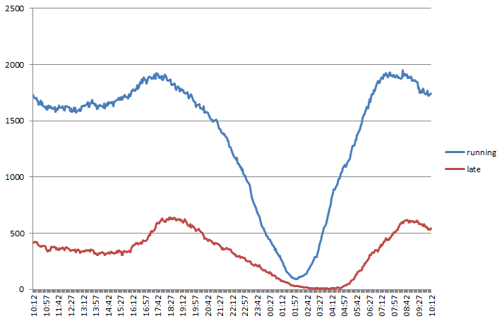
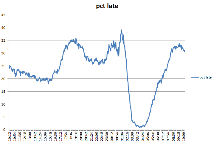
Going back to my initial comment about what we should be using this “supercomputing” capability for, it’s actually quite a difficult question to answer. “Fast Data” is probably a good answer though, as by doing complex analytics on things like real-time transport data we can predict where problems are likely to occur. Other forms of urban modelling are also good candidates, especially anything involving computations on large matrices.

Useful Links:

http://www.academia.edu/3770508/john_-L_Hennessy_and_David_A_Patterson_computer_architecture

https://openclnet.codeplex.com/

http://developer.download.nvidia.com/assets/cuda/files/reduction.pdf

http://www.amazon.co.uk/Heterogeneous-Computing-OpenCL-Revised-1-2/dp/0124058949/ref=sr_1_7?s=books&ie=UTF8&qid=1416491744&sr=1-7&keywords=opencl

https://www.nomisweb.co.uk/census/2011/bulk/rOD1

http://developer.amd.com/tools-and-sdks/opencl-zone/codexl/

POST Big Data Seminar and Information Age Reception

Today I’ve been attending the Parliamentary Office of Science and Technology (POST) seminar on Big Data after being interviewed by Stephen Hanley for the “Big and Open Data in Transport” POST Note back in July. It wasn’t held in the main Parliament building, but just around the corner from here:

IMG_20141106_173320

The first part of the seminar was a panel session discussing Big Data generally. The session was introduced by Adam Afriyie MP and chaired by Chris Tyler from POST. The panel was formed of Prof. Amanda Chessell (IBM), Prof. Carol Dezateux (UCL), Chris Fleming (Government Office for Science), Christopher Graham (Information Commissioner), Dr. Susan Grant-Muller (Leeds), Carl Miller (Centre for Analysis of Social Media), Matthew Rice (Privacy International), Dr. Emma Uprichard (Warwick).

After the Big Data session, there was a reception for the new “Information Age” exhibition at the Science Museum which launched a couple of weeks ago. Aside from Claude Shannon making an appearance, they had an analogue radio that you made work by connecting the components with wires, two robots that you could program via a “scratch” type web interface, plus a lot of old computer and communications hardware (Apple Newton!).

IMG_20141106_164436

The cute little robots are Arduino based with 3D printed bodies from an ABS printer rather than the PLA that we’re using with both our CASA MakerBots. In the picture you can also see the radio housed in the wooden box in the top left. The Science Museum demonstrators were really interested in our experiments with the HexBugs Spiders and Leap Motion control. I think we really need to do some more with robots in the future, but the Science Museum ones were running off 4xAA batteries, not the coin cells we kept having to replace when we were at Leeds City Museum.

The best part was the presentation by Sir Tim Berners-Lee about the origins and future of the World Wide Web:

IMG_20141106_154108

Afterwards, it was one of those moments when you really thought people would never stop clapping.

I also had an interesting conversation with Cubic Transportation Systems, the company that runs the UK Oystercard system. My initial question of, “how many people are there who use paper tickets and so get missed off the Oyster statistics”, had them wondering how to calculate it. The problem is that none of the data can actually give you this figure directly, and various estimates have been proposed. Aside from that, seeing their transport visualisation made me realise just how much real-time data we have in CASA and that we really should be doing more with it.

I’ve done nothing on real-time data since starting on Future Cities, so I decided to go back to the ANTS server and see if I could use the Network Rail data to answer the following Big Transport data question:

“If I pick any train at random in the UK, what is the probability that I pick a late running one?”

To cut a long story short, it’s about a 1 in 3 chance:

LateTrains05Nov06Nov2014 LateTrains05Nov06Nov2014_pct

The two graphs show data for the number of running trains, the number of late trains and the percentage late for 10am on 5th November 2014 to 10am on 6th November 2014.

That’s one application of “Big and Open Data in Transport”, which is exactly what what the POST note was about.

Useful Links:

http://www.parliament.uk/mps-lords-and-offices/offices/bicameral/post/post-events/

http://scratch.mit.edu/

http://www.arduino.cc/

And more on Hex Bug spiders:

http://www.geotalisman.org/2012/11/01/hex-bug-spiders-with-computer-vision/

http://www.geotalisman.org/2012/10/30/hacking-hex-bug-spiders/

http://www.geotalisman.org/2013/02/08/mark-1-spider-bee/